You just thought of a new idea for a trading system. You want to test it quickly to see if there is any value in it. The system requires a few technical indicators to be calculated based on past prices.
You are a momentum trader that is screening for the recent top performers in an index or sector.
You are a value investor that is screening for stocks that have had a recent 30% or greater drop in price that may be a good value stock to consider.
You are a long term investor that uses trailing stops on all of your positions. This helps you lock in your winners while giving them room to run. You must update these stops at the end of each trading day or week.
You are creating a trend following system. You are considering which markets that you want to trade in order to give the overall portfolio as much diversification as possible. To do this, you want to calculate the historical correlation between the markets that you are considering.
What do all of these traders have in common? In order to do the tasks that they are working on, they need access to historical price data. The most common type of historical price data is end-of-day (EOD) data for stocks, ETFs, and indices. This is a list of open, high, low, and closing prices. The daily trading volume is also typically included. This is one of the most common data sets that I use as a systematic trader. In this article, I’m going to show you how to download this information for free into Microsoft Excel.
Free Sources Available
There are two primary, free sources for this data – Yahoo Finance and Google Finance. We will take advantage of links on both websites that allow users to download this data into a csv file. These links have a specific URL structure that will allow us to automate this process for any stock or date range that we want. In this article, we are going to get this data from Yahoo. So let’s get started!
Get CSV File Download Link Address
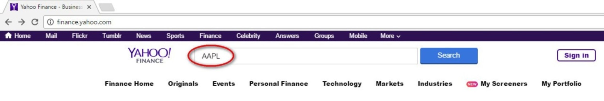
The first thing that we need to get is the specific csv file download link address for the stock and date range that we’re interested in. For this example, we are going to download three years of daily prices for Apple (Jan 1, 2014 to Dec 31, 2016). To do this, go to www.finance.yahoo.com, and then enter Apple’s ticker symbol AAPL into the Search for news, symbols or companies input box at the very top of the page.
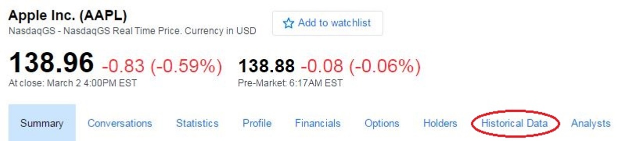
This takes us to the main Yahoo Finance page for Apple. Click on the Historical Data tab towards the top of the page.
We now see the complete list of historical prices for Apple. To get the specific date range that we want, click on the time period input and enter the start date (Jan. 1, 2014) and the end date (Dec. 31, 2016). Also notice that you can change the frequency of the prices to be Daily, Weekly, or Monthly prices. For this example, we will get the daily prices.
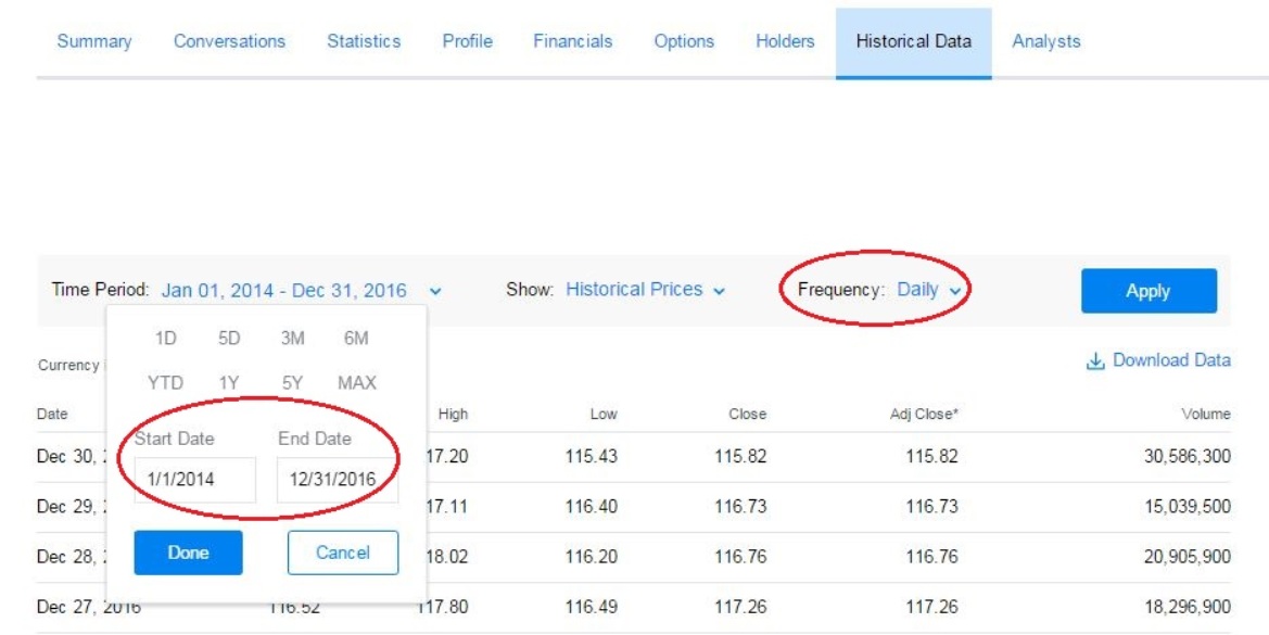
Once the inputs are correct, hit the Apply button. This updates the data listed on the page to only be for the date range and frequency that we entered. Notice just below the Apply button is a link that say’s Download Data. This is the download address that we want to get. If you left click on this, it will download the data displayed and save it as a comma-separated values or csv file.
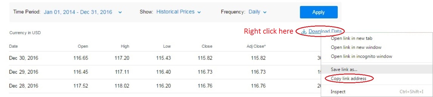
At this point, we could just hit the link, save the file, and then open it using Excel. But instead of doing this manually, we want to setup Excel to do this for us automatically – saving us a lot of time in the future. That is why we need the file download link. To get it, right click on the Download Data link and select Copy address link. If you paste this into a text editor, it should look something like this:
http://chart.finance.yahoo.com/table.csv?s=AAPL&a=0&b=1&c=2014&d=11&e=31&f=2016&g=d&ignore=.csv
Important note: If you do not see this Download data link, you will not be able to download the data for the stock you have entered. This can be the case for some stocks on foreign exchanges depending on your location.
Manually Get External Data into Excel
Now that we have the csv file download address, we can have Excel get this data and put it in the spreadsheet for us. The next few steps will vary slightly depending on the version of Microsoft Excel that you are using. I will describe the steps using Excel 2016.
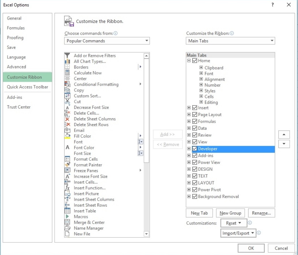
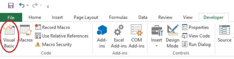
After opening Excel, we want to make sure that the Developer tab on the ribbon is visible. If this isn’t visible, go to Excel Options, Customize Ribbon, and make sure that the Developer main tab is selected.
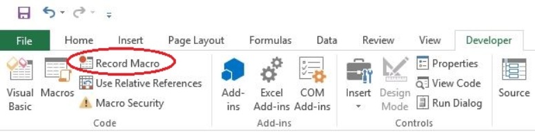
Now we want to start recording a macro. We will use the macro that we record in the next section to automate this process. To start recording a macro, go to the Developer tab on the ribbon and under the Code section, click on Record Macro.
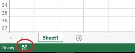
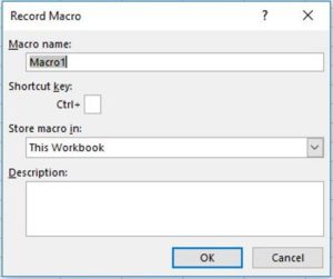
You can also start recording a macro by pressing the record macro button on the bottom left-hand corner of the Excel sheet. Either of these methods brings up a Record Macro prompt where you can enter the macro name, description, and location to store it. We will just use the default settings, so hit OK.
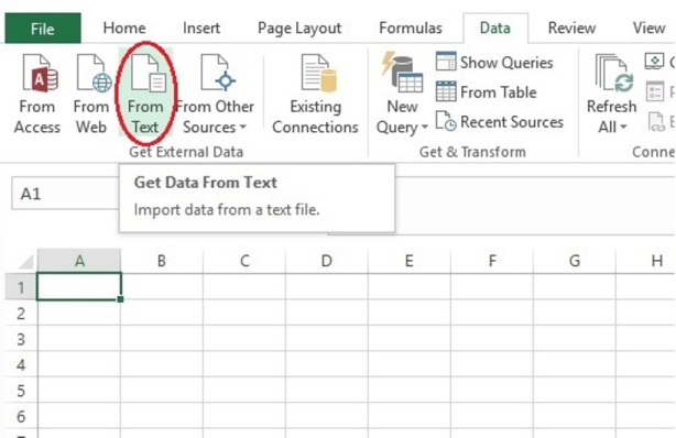
Now that a macro is recording, it will record the code for everything that we do inside of Excel. Go to the Data tab on the ribbon and under the Get External Data section, click on the From Text button.
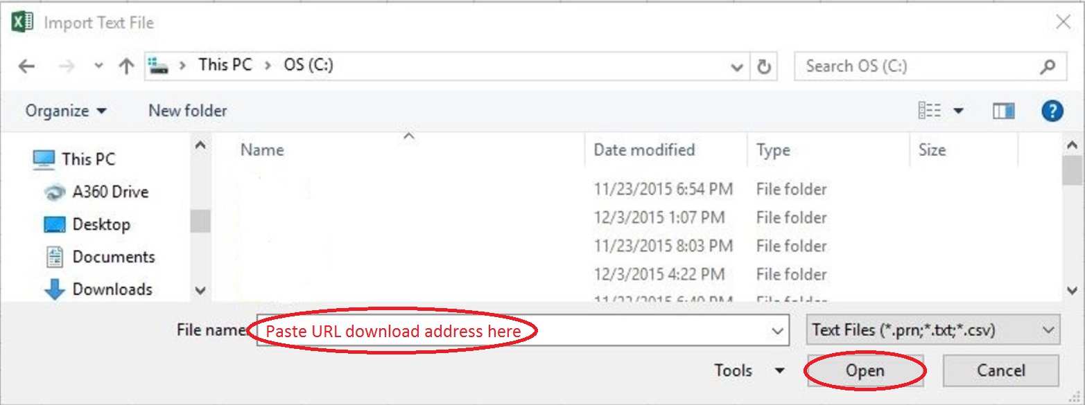
This brings up a window to import a text file. Under the file name, paste the URL download address that you copied, and then hit Open.
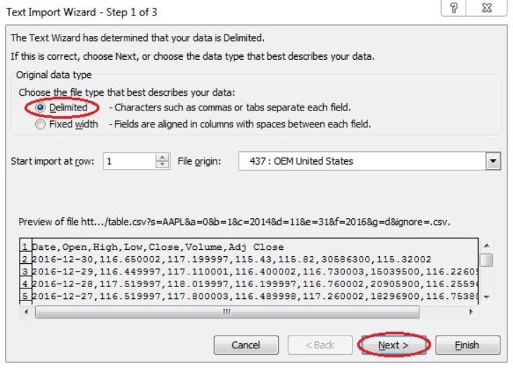
Excel will retrieve this csv file and determine that the data is delimited. This means that characters like commas separate each data value. This automatically brings up a Text Import Wizard to help properly put the data into the spreadsheet. Select that the data is Delimited, then hit Next.
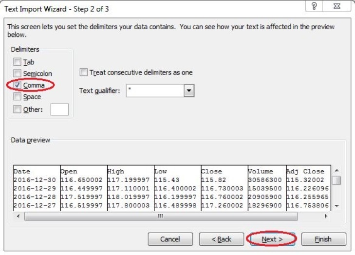
For step 2 of the import process, select the Comma to be the delimiter. You should see the data preview below properly separate the columns. Hit Next.
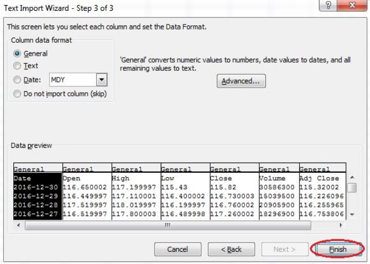
Step 3 allows you to set the format for each column of data. We will just use the default settings for now, so hit Finish.
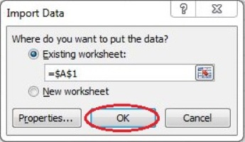
The import wizard now asks where you want to put the data. We will put it in the existing worksheet in cell $A$1. This is the default setting, so hit OK.
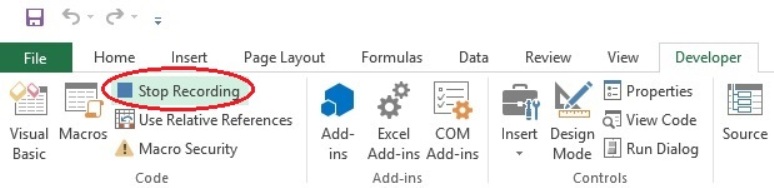
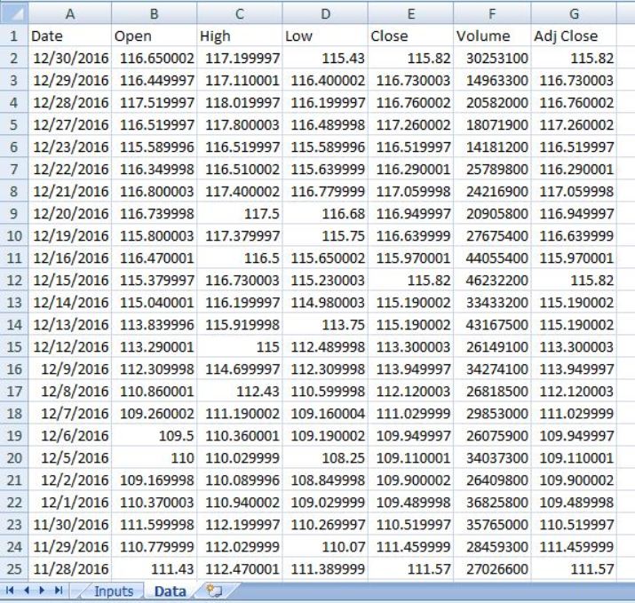
Now all of the price data that we wanted for Apple has been put into the spreadsheet. The column headers are Date, Open, High, Low, Close, Volume, and Adj Close. Now stop the macro that was recording in the background. Do this by going to the Developer tab on the ribbon and hit the Stop Recording button under the Code section.
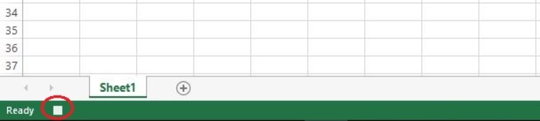
You can also hit the stop recording button at the bottom left-hand corner of the Excel sheet.
Automatically Get External Data into Excel
If we had to follow the steps outlined so far each time we wanted to get historical price data for a stock, it would be a very slow process. That is why we want to train Excel to do this for us automatically, regardless of the specific data that we want. We are going to create Excel macros to do this for us.
The next step is to look at the code that was recorded for us. To view the code, open the Visual Basic screen. You can do this by going to the Developer tab on the ribbon, and clicking on the Visual Basic icon in the Code section. Or a simple Windows shortcut is ALT + F11.
Once the Visual Basic screen opens, it should display the Macro1 code that was just recorded. If not, open the Modules folder in the Project Explorer on the left, and then double click on Module1. You should see code that looks like this:
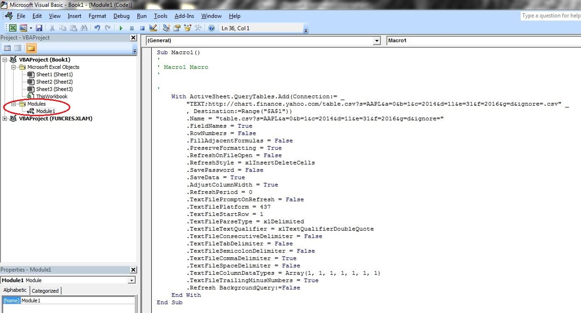
Looking at the code, you can see that with the active sheet, a query table from our text or csv file link address was added to range $A$1. This query table has many settings, but the important ones are:
- .TextFileParseType = xlDelimited
- .TextFileCommaDelimiter = True
- .Refresh BackgroundQuery:=False
These settings tell Excel that the text file imported into the spreadsheet has data that is delimited and separated by commas. The .Refresh method tells Excel to update the data on the sheet. Without this statement, the data would not be saved to the sheet.
This recorded code will be the basis for the automatic data download macro that we will write. But before we get too far into the programming, let’s setup our spreadsheets to make this process easier.
Input Sheet
First, we are going to setup a worksheet where we can enter the details for the data that we want to get from Yahoo. We’ll name this sheet, Inputs. At the bottom of the Excel workbook, right click on a sheet name and select Rename. Enter Inputs as the name.
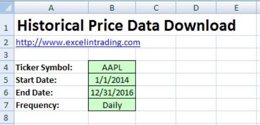
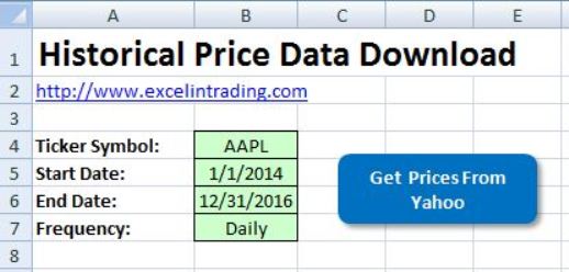
On this sheet, we will setup specific cells to be the macro inputs. We’ll put the input descriptions in column A and have the user enter the input values into column B. The descriptions are Ticker Symbol, Start Date, End Date, and Frequency. Put these descriptions in rows 4 through 7 in column A.
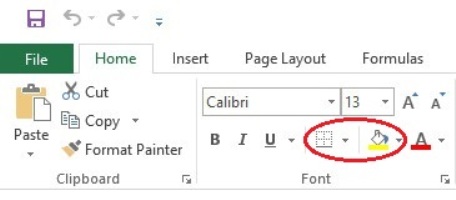
We want to make the input value cells stand out so that it is clear to the user where to enter this info. Let’s add borders around each input cell and fill the cells with a color to help show that they are user inputs. To add borders and change the cell fill color, first select the cells that you want to do this to. Then go to the Home tab on the ribbon and look under the Font section. The Borders and Fill Color options are beside one another. Click on the down arrows for each and select the borders and color that you want.
I like to use outside borders and a light green fill color to show that a cell is an input. Feel free to customize it to your liking. Here’s what my Inputs sheet looks like:
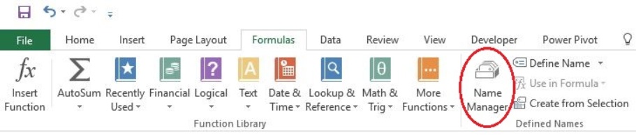
Now, we are going to make each of the input value cells a named range. This will make it easier to read our code and reference the correct cell in the code. This just means that we can use the cell’s name instead of the cell location (for example, ticker vs. B4). Start by clicking on cell B4 where we want to enter the ticker symbol. To create a named range, go to the Formulas tab on the ribbon and click on the Name Manager icon in the Defined Names section. Click New and then enter the desired name for the cell selected. Repeat this for all four inputs. We are going to use the following names:
- ticker (cell B4)
- start_date (cell B5)
- end_date (cell B6)
- frequency (cell B7)
Note that spaces are not allowed for named ranges. That is why we will use an underscore for a space. This is also a preferred way to name programming variables to make them more readable.
Data Sheet
Now we are going to create a worksheet to be the destination for the data download. We will name this sheet, Data. At the bottom of the Excel workbook, click on the New Sheet button. Or you can right click on an existing sheet, and select Insert. To rename the new sheet, right click on the sheet name, and select Rename. Enter Data as the name. That is all we need to do with this sheet for now.
Get Yahoo Historical Prices Sub-Routine
At this point we could make one macro to read the information from the Inputs sheet and download the desired data to the Data sheet. Instead, we will create one macro to read the user inputs and pass this information to another macro to handle the download process. The advantage to separate this and make the downloading process a single sub-routine is that we can take this block of code and easily use it in other programs that we will create later. Let’s create the Yahoo historical prices download macro first. Copy the code below and paste it into the code area of the Visual Basic screen. Make sure to scroll all the way to the right to get all of the code. Here’s the code:
Sub get_yahoo_historical_prices(ticker As String, start_date As Date, end_date As Date, frequency As String)
'sub-routine saves the historical price data for the ticker, dates, and frequency desired
'sub-routine saves the data on the active sheet when called

    'Get desired URL structure for Yahoo Finance
    Dim a As Integer: a = Month(start_date) - 1
    Dim b As Integer: b = Day(start_date)
    Dim c As Integer: c = Year(start_date)
    Dim d As Integer: d = Month(end_date) - 1
    Dim e As Integer: e = Day(end_date)
    Dim f As Integer: f = Year(end_date)
    Dim g As String
    If frequency = "Daily" Then
        g = "d"
    ElseIf frequency = "Weekly" Then
        g = "w"
    ElseIf frequency = "Monthly" Then
        g = "m"
    Else
        MsgBox ("Invalid frequency input for " & ticker & "." & vbNewLine & _
            "Frequency input was set to : " & frequency & vbNewLine & _
            "Frequency input must be Daily, Weekly, or Monthly.")
        Exit Sub
    End If

    Dim yahoo_url As String: yahoo_url = "http://chart.finance.yahoo.com/table.csv?" & _
        "s=" & ticker & _
        "&a=" & a & _
        "&b=" & b & _
        "&c=" & c & _
        "&d=" & d & _
        "&e=" & e & _
        "&f=" & f & _
        "&g=" & g & _
        "&ignore=.csv"

    'Save data from csv file to the active sheet
    With ActiveSheet.QueryTables.Add(Connection:="TEXT;" & yahoo_url, Destination:=Range("$A$1"))
        .Name = ticker
        .TextFileParseType = xlDelimited
        .TextFileCommaDelimiter = True
        .Refresh BackgroundQuery:=False
    End With

End Sub
So let’s walk through this code to better understand what it is doing. First off, the code defines the variables a, b, c, d, e, f, and g. These are used to help get the specific Yahoo download link address based upon the inputs to the sub-routine. Here is the link for the example that we used earlier:
http://chart.finance.yahoo.com/table.csv?s=AAPL&a=0&b=1&c=2014&d=11&e=31&f=2016&g=d&ignore=.csv
Let’s break this down to better understand the URL structure:
http://chart.finance.yahoo.com/table.csv?
s=AAPL&
a=0&
b=1&
c=2014&
d=11&
e=31&
f=2016&
g=d&
ignore=.csv
Notice that s is set to the ticker symbol for Apple, or AAPL. It’s not obvious, but the letter a is set to the start date’s month minus 1. The letter b is set to the start date’s day, and letter c is set to the start date’s year. Similarly, letter d is set to the end date’s month minus 1, e is set to the end date’s day, and f is set to the end date’s year.
Letter g is set to d. This is because the frequency of the data was set to Daily. If this was set to Weekly, g would be equal to w. If the frequency was Monthly, then g would be equal to m.
The last part of the URL is ignore=.csv. This will be the same, regardless of the data desired.
So, this is exactly what the code is doing. It defines letters a through f based on the start and end date inputs. Then it defines g based on the frequency input. Notice that g must be Daily, Weekly, or Monthly. If this input is not one of these values, then the code will give a message to the user stating that the frequency input wasn’t valid and then exits the sub-routine.
After letters a through g are defined, the code can define what the specific Yahoo download address should be. This is saved to the variable yahoo_url.
Now that the code knows the link to the csv text file download, it uses the same block of code that we recorded earlier to add a query table to the active sheet. This is what actually retrieves the data from Yahoo’s website and saves it on the active sheet. It uses the yahoo_url variable instead of the hard coded address that we copied. It also only has the query table settings that are necessary.
Yahoo Prices Sub-Routine
Now that we have a sub-routine to get the data that we want, we need another sub-routine to get the user inputs and pass this information to the previous sub-routine. We’ll call this new sub-routine yahoo_prices. Copy the code below and paste it into the code area of the Visual Basic screen. Here’s the code:
Sub yahoo_prices()
'sub-routine retrieves the user inputs from the "Inputs" sheet and passes this into the Get_Yahoo_Historical_Prices function

 'Save necessary input variables
 Dim ticker As String: ticker = Sheets("Inputs").Range("ticker").Value
 Dim start_date As Date: start_date = Sheets("Inputs").Range("start_date").Value
 Dim end_date As Date: end_date = Sheets("Inputs").Range("end_date").Value
 Dim frequency As String: frequency = Sheets("Inputs").Range("frequency").Value

 'Activate appropriate sheet to put price data
 ThisWorkbook.Sheets("Data").Activate
 'Delete any data currently on the sheet
 Cells.Delete

 'Call the yahoo sub-routine
 Call get_yahoo_historical_prices(ticker, start_date, end_date, frequency)

End Sub
So what it is this code doing? First, it defines the four user inputs from the Inputs sheet. It references the named ranges on this sheet that we created earlier. Next, it activates the Data sheet and deletes any values on the sheet. This makes sure that no previously download data will accidentally be left on the sheet. Last, it calls the get_yahoo_historical_prices sub-routine that we previously created, and it passes the four user inputs into the sub. This call statement will run the other sub-routine.
Test It Out!
Let’s test out this new macro. Go to the Inputs sheet and enter the inputs in the appropriate cells if you haven’t already. To make it easier to call our macros, let’s add a button on the “Inputs” sheet that we will link to this sub-routine. That way if we want to run the macro, we can enter all of the inputs and just push this button.
There’s several ways to do this. We will go the Insert tab on the ribbon and click on Shapes under the Illustrations section. Under Rectangles, we will select the Rounded Rectangle. Click on the sheet, and drag the cursor from the top left to the bottom right to create a rectangle. Right-click on this and click on Edit Text. Enter Get Prices From Yahoo. Now right-click on the rectangle again, and click on Assign Macro. Select the yahoo_prices sub that we created. Here’s what my Inputs sheet looks like now:
Click on the new macro button. It should run the yahoo_prices sub-routine and download the historical prices to the Data sheet. Here’s what the Data sheet should look like:
Awesome! We just downloaded historical price data into Excel. Enter some different ticker symbols, dates, and data frequency, and test it out.
So to conclude, if you would like to download this Excel workbook for free, you are in luck. You can get it below with several extra features also thrown in, including the ability to automatically download the data for a list of stocks. In the next article, I’ll show you how to download this data from Google Finance.